Wrong By Design

STAT 20: Introduction to Probability and Statistics

Agenda

• Concept Questions
• Practice Problems

Concept Questions

Concept Questions 1 and 2

The following two questions are based on the diagram below. The diagram corresponds to a one-sided hypothesis test that uses the following null hypothesis: \(H_0: \mu = 1\)

If \(H_A\) represents a specific version of the alternate hypothesis that is true, what is the power of this test?

01:00

What is the p-value of this test?

01:00

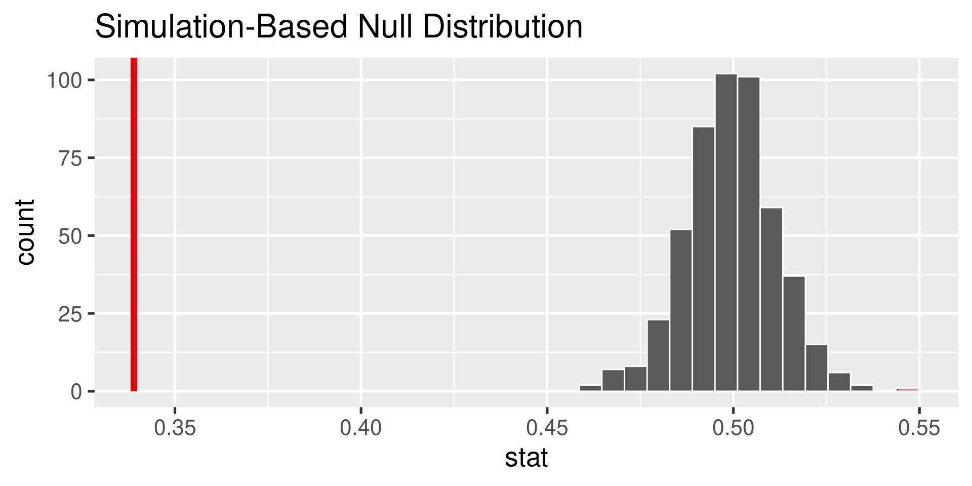
Instead of constructing a confidence interval to learn about the parameter, we could assert the value of a parameter and see whether it is consistent with the data using a hypothesis test. Say you are interested in testing whether there is a clear majority opinion of support or opposition to the project.

What are the null and alternative hypotheses?

01:00

The null is the p = .5 and the alternative is that p != .5.

This brings up a good discussion of one- and two-tailed tests. When students share their answers, you can draw a picture of a null distribution on the board with the observed statistic as a vertical line and consider how the p-value calculation would change depending on the alternative hypothesis.

This also brings up a discussion of the link between hypothesis tests and confidence intervals. Below the picture of the null distribution on the board, you could draw a bootstrap distribution centered on the vertical line of the observed statistic. In the HT setting, you consider the location of the statistic relative to the null distribution. In making a decision with a CI, you consider the location of the parameter relative to the bootstrap distribution (or more generally, the sampling distribution of the statistic).

library(tidyverse)
library(infer)
library(stat20data)

ppk <- ppk %>%
  mutate(support_before = Q18_words %in% c("Somewhat support", 
                                          "Strongly support",
                                          "Very strongly support"))

library(tidyverse)
library(infer)
library(stat20data)

ppk <- ppk %>%
  mutate(support_before = Q18_words %in% c("Somewhat support", 
                                          "Strongly support",
                                          "Very strongly support"))
obs_stat <- ppk %>%
  specify(response = support_before,
          success = "TRUE") %>%
  calculate(stat = "prop")

library(tidyverse)
library(infer)
library(stat20data)

ppk <- ppk %>%
  mutate(support_before = Q18_words %in% c("Somewhat support", 
                                          "Strongly support",
                                          "Very strongly support"))
obs_stat <- ppk %>%
  specify(response = support_before,
          success = "TRUE") %>%
  calculate(stat = "prop")
obs_stat

Response: support_before (factor)
# A tibble: 1 × 1
   stat
  <dbl>
1 0.339

null <- ppk %>%
  specify(response = support_before,
          success = "TRUE") %>%
  hypothesize(null = "point", p = .5) %>%
  generate(reps = 500, type = "draw") %>%
  calculate(stat = "prop")

null <- ppk %>%
  specify(response = support_before,
          success = "TRUE") %>%
  hypothesize(null = "point", p = .5) %>%
  generate(reps = 500, type = "draw") %>%
  calculate(stat = "prop")
null

Response: support_before (factor)
Null Hypothesis: point
# A tibble: 500 × 2
   replicate  stat
   <fct>     <dbl>
 1 1         0.490
 2 2         0.528
 3 3         0.483
 4 4         0.513
 5 5         0.499
 6 6         0.502
 7 7         0.498
 8 8         0.495
 9 9         0.511
10 10        0.491
# ℹ 490 more rows

null <- ppk %>%
  specify(response = support_before,
          success = "TRUE") %>%
  hypothesize(null = "point", p = .5) %>%
  generate(reps = 500, type = "draw") %>%
  calculate(stat = "prop")
visualize(null) +
  shade_p_value(obs_stat, direction = "both")

What would a Type I error be in this context?

Answer: Concluding that there is a clear majority when in fact there is an even split.

01:00

What would a Type II error be in this context?

Answer: Concluding that there is an even split when in fact there is a clear majority.

After the previous question, students should get this quite easily.

01:00

Hypothesis Testing Review

One goal for today

Learn why we don’t accept the null hypothesis.

What is it good for?

Hypothesis tests have been shown to be valuable contributors to science (p < .05) but are sometimes abused (p < .05).

• Used to assess the degree to which data is consistent with a particular model.
• The most widely used tool in statistical inference.

Step 1

Lay out your model(s).

\(H_0\): null model, business as usual
\(H_A\): alternative model, business not as usual

• Hypotheses are statments about the TRUE STATE of the world and should involve parameters, not statistics.
• Hypotheses should suggest a test statistic that has some bearing on the claim.
• The nature of \(H_A\) determines one- or two-sided tests; default to two.

Step 2

Select a test statistic that bears on the null hypothesis.

• \(\bar{x}\)
• \(\hat{p}\)
• \(m\)
• \(r\)
• \(b_1\)

• \(\bar{x}_1 - \bar{x}_2\)
• \(\hat{p}_1 - \hat{p}_2\)
• \(m_1 - m_2\)
• \(\chi^2\)
• The list goes on…

Step 3

Construct the appropriate null distribution.

1. Permutation (when null = "independence")
2. Simulation (when null = "point")
3. Normal Approximation

Step 4

Calculate a measure of consistency between the observed test statistic (the data) and the null distribution (i.e., a p-value).

• If your observed test stat is in the tails
  • low p-val
  • data is inconsistent with null hypothesis
  • “reject null hypothesis”.

• If your observed test stat is in the body
  • high p-val
  • data is consistent with the null hypothesis
  • “fail to reject the null hypothesis”.

What can go wrong?

Decision Errors

Grammar of Graphics review

What geometries are in use in this graphic?

A simplified model

UHS tests a sample of the Cal community every week and monitors the positivity rate (proportion of tests that are positive). Assume this is a random sample of constant size and that the test is perfectly accurate. Let \(p\) be the positivity rate.

\(H_0\) \(\quad p = 3\%\)

The incidence of COVID at Cal is at a manageable level.

\(H_A\) \(\quad p > 3\%\)

The incidence of COVID at Cal is at an elevated level.

Decision protocol: if there is a big enough spike in a given week, shift classes to remote.

Decision Errors

Build this plot up slowly on the board. Recommended order:

1. Null dist. If the null distribution is true, than we’d observe p-hats from the null distribution on the left.
2. Vertical line that demarcates rejection region from do-not-reject region.
3. If we use alpha = .05, what is the chance that we generate a p-hat in the reject region? .05
4. Alt dist. What if instead the alt were true with this particular p (draw alt dist on right)?
5. If we’re generating p-hats from the alt distribution, what’s the chance we’d generate one that looks like it’s from the null (i.e. in the fail-to-reject region)?
6. If we’re generating p-hats from the alt distribution, what is the chance we’d notice i.e. that change that we’d reject the null?

This can lead into a discussion of what effects power:

What would we have to do to this graphic to increase the area under the curve that represents power?

1. increase alpha
2. bring the distributions farther apart (increase effect size)
3. decrease the spread of the distributions (increasing sample size is the approach they’ll be familiar with. this is also where clever methods in survey sampling and experimental design come in: blocking and stratification)

Error Rates and Statistical Power

Decision Errors Rates

What affects the error rates?

• Sample size, \(n\): with increasing \(n\), the variability of the null distribution will decrease.

• Changing \(\alpha\): decreasing \(\alpha\) will decrease type I error but increase type II error.

• Increasing effect size: change data collection process to separate the distribution under \(H_A\) and decrease type II error.

  • Ex: If you’re testing whether a pain medicine provides pain relief, only conduct the test if using a medicine that you expect to have cause a dramatic decrease in pain.

Consider a setting where the Cal UHS testing system observes a positivity rate of 3.5% in a one week interval, double the previous week. Administration needs to decide whether or not to move to remote learning. Which error would be worse?

A. Moving to remote instruction when in fact the true number of cases on campus is still low.

B. Failing to move to remote instruction when in fact the true number of cases on campus is elevated.

01:00

Statistical Power

Power is the probability that you will reject the null hypothesis if it is in fact false.

\[ P(\textrm{reject } H_0 | H_0 \textrm{ is false}) \]

The more power, the higher the probability of finding an effect.

This is an example of how low-power studies resulted in a failure to detect that masks were in fact helpful. The plot on the next page is pretty tricky to interpret, so only show it if you’ve skimmed the paper and are ready to talk through the plot.

One goal for today

Learn why we don’t accept the null hypothesis.